
Analysis of elementary stress/dynamic analysis of the total stress/ dynamic analysis of effective stress (liquefaction analysis) program
Dynamic effective stress analysis for ground(UWLC) Ver.2
Initial Release:2004.04.05 / Latest Ver.:2011.10.28
- USD6,300
English Version Ver.2
Initial Release:2006.03.28 / Latest Ver.:2016.12.16
- USD12,600
Related products and services:
Geotechnical analysis support service Trial Version
Program Overview
This program is to analyze dynamic land transformation using finite element method (FEM). Taking into consideration the method of elastic theory based on effective stress, excessive pore water pressure which occurs during earthquakes and the declining of stiffness, it is possible to calculate land transformation by the hour.
This program can be applied to investigating the stability of earth structures (banks or raised mounds), the lift of underground structures, and the dynamic interrelation between an earthquake and structures.
Another program with function to decide parameters in liquefaction is attached. It allows you to input in a CAD style making easy creation possible. It also accepts reading from SXF files.
File cooperation with GeoFEAS2D and import of terrain data exported from Flexible structure sluiceway is possible.
The analytic core of this program makes use of the land analysis program by Prof. Ugai and his research laboratory at Gunma University. They are involved in advanced analytic theory and have made brilliant achievements. This program is jointly developed by our company, which is engaged in the development of the prepost part, and the university.
Functions and Features
Analysis features
-
- It is possible to set parameters in liquefaction by carrying out simulation for element test.
- Identification analysis program by the optimization method is attached so that entered parameter can be set from experiment data.
- Parameters of sand structure model (PZ-sand) can be estimated from N value of the standard penetration test
- It conducts one-dimensional and two-dimensional analyses.
- It is possible to carry out the dynamic analysis of total stress method and of effective analysis (analysis in liquefaction).
- Applied elements for total stress method (ignoring water pressure) and applied elements for effective stress method (considering water pressure) can be used in mixed situations.
- Dynamic analysis of earth and water successively formed on the assumption of water penetration.
- Plenty of structure models of land (eight categories) are available and these can be used freely.
- It adopts BFGS, which is a line search for calculating convergence.
- Stable analysis by making automatic adjustment in time steps of dynamic analysis.
- Supports simultaneous vertical and horizontal excitation
Scope and application
-
- Investigation of the dynamic interrelation between land and building structures by using the total stress method.
- Investigation of stability at an earthquake including earth structures(river banks, for example).
- Investigation of the lift of structures in the liquid land.
- Investigation of the method against.
- Dissipation of Excess Pore Water Pressure Method like Gravel drain method are supported.
- Simulation of experiments such as a centrifugal vibration experiment or a large-sized vibration table.
- Judgment of minute liquefaction by means of one-dimensional response analysis during earthquakes.
- Method by structures
- Consolidation method
- Sand compaction pile method
- Gravel drain method
- 2D FEM model can be created by simple CAD like operations.
- CAD data (SXF) importing is supported.
- Mesh division (block division method)
- Simple creation of 1 dimension analysis model
- Mesh data export
- Table of material parameter
Example of available liquefaction countermeasures
Analysis functions Initial stress analysis 
All stress analysis Dynamic analysis All stress analysis Valid stress analysis (liquefaction analysis)
Flow of analysis model creation 
Theory of analysis
-
- Linear elastic model
- Laminated elastic model
- Elastic and complete plastic model
- Modified Ramberg-Osgood model (RO model)
- Modified Hardin-Drnevich model (HD model)
- Ugai-Wakai model (UW-Clay model)
- Pastor-Zienkiewicz model for sand (PZ-Sand model)
- Pastor-Zienkiewicz model for clay (PZ-Clay model)
- Mass matrix---Concentrated mass matrix or consistent mass matrix
- Damping matrix---Concentrated damping matrix or consistent damping matrix
- Explicit method---forward calculus of finite differences.
- Implicit method---Newmark-β method / HHT-α method / WBZ-α method / Generalized-α method
1. Factor library
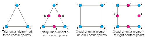
(1) Distortion element on a plain surface
It is possible to define four elements: triangular element at three contact points,triangular element at six contact points, quadrangular element at four contact points and quadrangular element at eight contact points.
(2) Beam element
It is possible to define primary beam element.
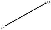
(3) Axial spring element
Definition is given at two contact points. The length of the spring must be 10 - 5 m or longer.
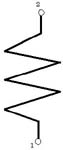
(4) Shearing spring element
Definition is given at two contact points. The length of the spring must be 10 - 5 m or longer.
(5) Mass element centered on one contact point
Definition is given at one contact point.
(6) Damper element
Definition is given at two contact points. The element indicates declining in the axial and shearing directions.
2. Constituent models
(1) Distortion element model on a plain surface
(2) Beam element model
Linear elastic model or bilinear model can be used as stability feature in the beam element.
(3) Spring element model
Linear elastic model or bilinear model can be used as stability feature in the axial direction and shearing spring element. It is also possible to define the concentrated mass at contact points at both the ends of spring.
3. Mass matrix and damping matrix
(1) Concentrated matrix and consistent matrix
In this program it is possible to choose either concentrated matrix or consistent matrix to be applied to mass matrix and damping matrix.
However, you have to use consistent damping matrix if you regard Rayleigh damping as viscous damping.
(2) Rayleigh damping
Energy damping covers viscous and fugitive damping as well as aftereffect damping.
In this program Rayleigh damping can be considered to be viscous damping.
4. Dynamic equation and simultaneous equation
(1) Degitizing and integral calculus in dynamic equation
(2) Solution of simultaneous equation
This program stores into memory total rigid matrix by means of skyline method.
As solution of simultaneous equation it adopts LDLT resolving method which is changed from Gaussian elimination.
Identification analysis of the material parameter
-
The identification analysis program is available as an accessory program. The optimal parameters obtained from the program can be read into the material property settings in UWLC itself. For the soil constitutive model UW-Clay, the determined parameters can be read into the conventional element test simulation program to simulate stress strain curves, etc.
▲Identification analysis by
the optimization method
Estimate the sand structure model parameter from N value
-
As a soil model for liquefaction, elasto-plasticity and PZ-Sand (Pastor-Zienkiewicz) are available in UWLC. Until now, it was necessary to obtain the angle of the internal friction and the deformation coefficient and to calculate the parameter to define the alternation line in advance in order to determine the parameter. Alteration line defines shift in constriction and swelling of sand dilatancy in the stress space. Sand constricts if Mohr's stress circle is within the alteration line, and if not, it swells. Parameters can be estimated from N-value with this function now.
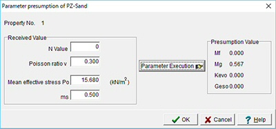
▲PZ-sand parameter estimation
Representational function of the analyzed results
-
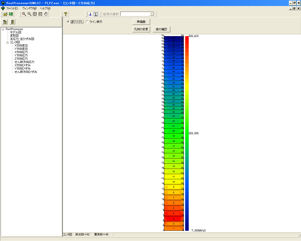
It supports displaying model diagram, distortion diagram, time history diagram (displacement, speed, acceleration, stress, distortion, excessive pore water pressure, beam section force), drawing of characteristic force of restitution, responsive spectrum diagram, Fourier spectrum diagram, contour diagram, diagram of cross-section force, main stress/main distortion, animation, and value output (node, element, beam section force).
Literature introducing UWLC
-
UWLC is introduced as an example and overview of dynamic deformation analysis method.
"Design and construction manual about high-standard embankment" (published in March 2000 by the Foundation for Riverfront Improvement and Restoration)
Enhancing CIM features of Geo technical Analysis series
-
We enhanced the CIM (Construction Information Modeling) function of various products in the geotechnical analysis series. The programs can cooperate terrain data or data created with each geotechnical analysis programs smoothly. Data linkage using terrain data file (*.GF1) Geotechnical Finite element Elastoplastic Analysis Software (GeoFEAS)2D Ver.4
The amount of displacement exported to Flexible structure sluiceway design for further analysis
By importing results of ground deformation analysis (settlement / horizontal displacement distribution) into the "Flexible structure sluiceway design", the level2 seismic test for the longitudinal direction can be performed.
GeoFEAS2D

Flexible structure sluiceway design
It can model only ground that a surrounding ground effect analysis is conducted in the Temporary sheathing work design. The ground deformation can be calculated by giving the wall displacement as the forced displacement.Dynamic effective stress analysis for ground(UWLC)Ver.2
Acceleration rate exported to Slope stability analysis for further analysis
When applying the Newmark method to high embankments with a height of about 30 m or more, it is necessary to input the response acceleration waveform of the slip soil mass as the ground motion.
Data linkage between "Dynamic effective stress analysis for ground (UWLC)" and "Slope stability analysis" corresponds to the Newmark method analysis calculated by using the response acceleration waveform.
The level2 seismic stability calculation for high embankment and large embankment.
UWLC
Slope stability analysis
2-D seepage analysis(VGFlow2D) Ver.3
Water line data exported to GeoFEAS2D
VGFlow2D
GeoFEAS2D
Water level data exported to UWLC
Water line and potential line exported to Slope stability analysis
Saturated / unsaturated seepage FEM analysis results can be reflected by file linkage (*.PRS [water line], *.PTN [isopotential line]).GeoFEAS Flow3D (limited to the seepage analysis)
Water level data imported to LEM3D
Analysis results computed with GeoFEAS Flow3D (limited to the seepage analysis) or third party's product can be imported to 3-D slope stability analysis(LEM). It creates underground water level required for landslide analysis and enables the 3D slope stability analysis.
VGFlow3D
LEM3D


Application criteria and References
-
- マトリックスと有限要素法[改定新版] (O.C. Zienkiewicz, R.L.Taylor, Kagaku Gijutsu Shuppan, Inc.)
- 地盤技術者のためのFEMシリーズ 1 はじめて学ぶ有限要素法 (The Japanese Geotechnical Society)
- 地盤技術者のためのFEMシリーズ 2 有限要素法がわかる (The Japanese Geotechnical Society)
- 地盤技術者のためのFEMシリーズ 3 弾塑性有限要素法をつかう (The Japanese Geotechnical Society)
- 地盤液状化の科学 (Fusao Oka, Kinmiraisha Company)
- 動的解析と耐震設計[第2巻] 動的解析の方法 (The Japanese Geotechnical Society)
- Chung, J. and G.M. Hulbert, A Time Integration Algorithm for Structural Dynamics with Improved Numerical Dissipation: The Generalized-α Method, ASME, Journal for Applied Mechanics, 60, 371-375, 1993.
- Hilber, H.M., T.J.R. Hughes and R.L. Taylor, Improved Numerical Dissipation for Time Integration Algorithms in Structural Dynamics, Earthquake Engineering and Structural Dynamics, 5, 283-292, 1977.
- Hughes, T.J.R., Analysis of Transient Algorithms with Particular Reference to Stability Behavior, Computational Methods for Transient Analysis, North-Holland, 67-155, 1983.
- Hulbert, G.M. and I. Jang, Automatic Time Step Control Algorithms for Structural Dynamics, Computer Methods in Applied Mechanics and Engineering, 126, 155-178, 1995.
- Newmark, N. M., A Method of Computation for Structural Dynamics, ASCE, Journal of the Engineering Mechanics Division, 85, EM3, 67-94, 1959.
- Wood, W.L., M. Bossak and O.C. Zienkiewicz, An Alpha Modification of Newmark's Method, International Journal for Numerical Methods in Engineering, 15, 1562-1566, 1981.
Price
Product Price
-
■Product Price
Product
Price
Dynamic effective stress analysis for ground(UWLC) Ver.2 USD6,300 Dynamic effective stress analysis for ground(UWLC) English Version Ver.2 USD12,600 ■Price of Floating License
Paying 40% of the product price allows anyone to use the product on any PC anywhere in the world.
Product
Price
Dynamic effective stress analysis for ground(UWLC) Ver.2 USD2,520 Dynamic effective stress analysis for ground(UWLC) English Version Ver.2 USD5,040
Price of Subscription Service Contract
Price of Subscription Service Contract
-
■Support information
-Software upgrade -Technical inquiry (Email, Tel)
-Download service -Maintenance and update notifications via email
* We are sequentially making a transition from the maintenance-support service to [Subscription Service] from April 1, 2016 in order to enhance support for diverse product usage and to reduce license management cost.Product Subscription cost
of first yearSubscription cost
of subsequent years
(annual cost)Subscription (Dynamic effective stress analysis for ground(UWLC) Ver.2) Free USD2,520 Subscription (Dynamic effective stress analysis for ground(UWLC)
English Version Ver.2)USD5,040 Subscription (Dynamic effective stress analysis for ground(UWLC) Ver.2 Floating) USD3,528 Subscription (Dynamic effective stress analysis for ground(UWLC)
English Version Ver.2 Floating)USD7,056
Price of Rental License / Floating License
■Rental license : Short term licenses available at a low price
■Rental floating license : After web activation, anyone can use the products on any PC anywhere in the world.
■Rental access : You can increase the number of licenses you own and use these additional licenses for a specific period of time (1 month to 3 month) at your discretion. We will later send you an invoice based on your usage log. The advance application is 15% off of the regular rental license price. Please place an order from User information page.
*Rental / Floating Licenses were introduced on September 2007 to enhance user experience and convenience of our products.
*Duration of Rental / Floating Licenses cannot be changed after starting these services. Re-application is required to extend the rental and floating license duration.
Rental license / Rental floating license
-
■Rental License
Product 2 month 3 month 6 month Dynamic effective stress analysis for ground(UWLC) Ver.2 USD2,835 USD3,339 USD4,095 Dynamic effective stress analysis for ground(UWLC)
English Version Ver.2USD5,670 USD6,678 USD8,190 ■Rental Floating License
Product 2 month 3 month 6 month Dynamic effective stress analysis for ground(UWLC) Ver.2 USD4,725 USD5,607 USD6,930 Dynamic effective stress analysis for ground(UWLC)
English Version Ver.2USD9,450 USD11,214 USD13,860
Academic Price
An Academic License can be provided for educational purposes and used by teachers, lecturers, academic researchers, and students.
Academic Price
-
Product Academic Price Dynamic effective stress analysis for ground(UWLC) Ver.2 USD2,170 Dynamic effective stress analysis for ground(UWLC) English Version Ver.2 USD4,340
Version Update History
Version Update History
-
■The version upgrade and revision upgrade (without charge) contents are listed as following.
Dynamic effective stress analysis for ground(UWLC) English Version Ver.2 Version Release date Update contents 2.00.00 16/12/16 - Identification analysis program by the optimization method is attached.
- Supporting topographic data for ground analysis (*.GF1).
- Importing DXF and DWG file.
- "CAD file import" by pre part supports AutoCAD2007 file format.
- Semi automatic setting of entered parameter (PZ-sand)
- Vibrations in the vertical direction and horizontal direction can be supported at the same time.
- When creating a model, it is now possible to determine whether the distance between points is close or not.
- Added a function to cancel all blocks in [Create_model] - [Decide] tab
- Added a command to set the selected node as origin in [Create_model] - [Create] tab.
- Added "Open sample data file" in the File menu.
Product Operation Environment
Product Operation Environment
-
OS Windows 8 / 10 / 11 CPU Pentium III 800MHz or higher (Pentium IV 3.0GHz or higher is recommended) Required memory (including OS) Greater than 512MB is recommended. Required Disk Capacity Greater than 120MB. Analysis requires 500 MB to a few GB according to model size. Display (Image Resolution) Greater than 1024×768 Input data extension FUD File export No. Refer to the help as for analysis part export file. Cooperation with other products <Loading>
Chart (SXF, DXF)
Linkage data with ground analysis (USD)
ToLipographic data for ground analysis (GF1)
<Linkage with>
Slope stability analysis
Order / Contact Us
Order / Contact Us
-
■ Inquiry
Contact us from Sales inquiry or email to ist@forum8.co.jp or forum8@forum8.co.jp
Display Samples

▲Model making
▲Entering parameter of the pre part
▲Example of one-dimensional analytic model
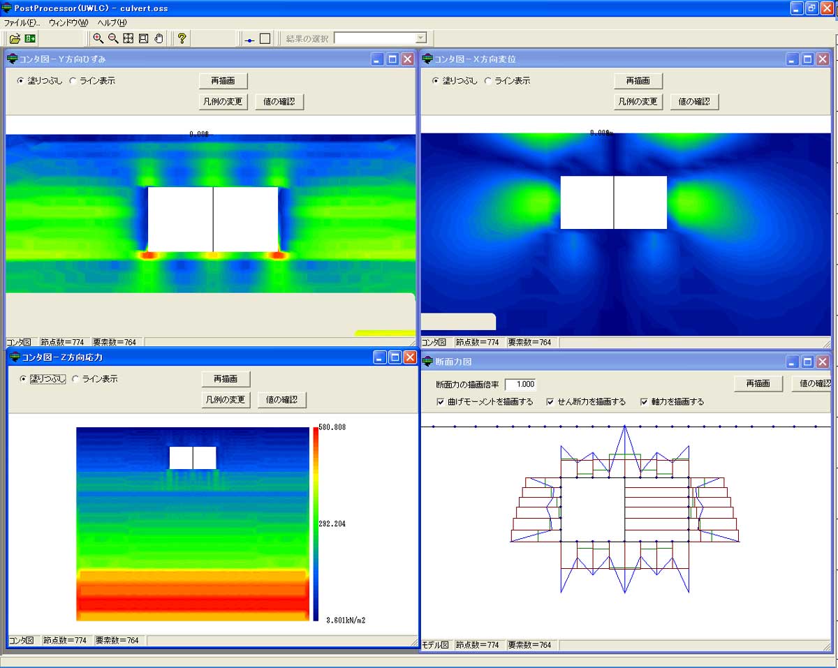
▲Coupled model with structures
(BOX culvert)
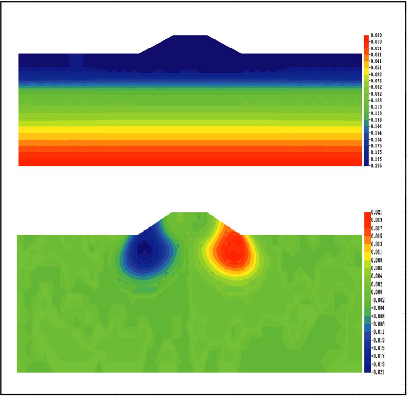
▲Examination of the embankment liquefaction
▲Examination both of the ground and the box culvert
▲Excessive pore water pressure rate
(Analysis of two-dimensional liquefaction)
▲Features of force of restitution (τ-σcurve)
▲Satisfied function of animation
▲Animation for transformation diagram (Bank model)
▲Identification analysis by the optimization method
▲Element test simulation program

▲Read-in function of the SXF drawing data
1. Function / Overview
- Can we analyze with the seismic wave of hachinohe wave?
-
For the horizontal acceleration data, the arbitrary seismic wave including hachinohe wave can be used.
If you want to adjust the maximum value of the acceleration, you can use the menu to adjust the input waveform in the window for loading the seismic wave file in the setting of loading stage.
In general, the method that K-NET developed in NIET (National Research Institute for Earth Science and Disaster Prevention) is used to obtain the seismic wave. - Can we perform comparative analysis for the basic input waveform and the ground surface output waveform?
-
Yes, it is possible. You can output the data into excel file format for comparisons.
- Can we extract the maximum value of horizontal force, foundation pile stress, and ground surface of acceleration based on the whip swing phenomenon of the tower?
-
To extract the maximum value of the horizontal force in the tower, please model the tower with the beam member and check the input in the time-history to detect the maximum value. The foundation pile is processed similarly. Please display the time-history diagram, and right mouse click placing the cursor over the screen. The menu which has the graph edit function is displayed, and the data is exported in excel format. It is suggested that you should detect the maximum value from the data and verify it in the section force diagram of that time. It is better to draw the time-history diagram separately as the maximum value of NMQ (shear force) does not necessarily occur at the same time.
The acceleration of the ground surface is processed in the same way as the above mentioned section force. Please focus on the arbitrary node point and export the data after drawing the time-history diagram to detect the maximum value (absolute value). - Can we export the acceleration waveform as the text file?
-
Yes, perform a right mouse click on the graph after displaying the time-history waveform to show Edit menu then select Download, and the text file.
- Can we perform self-weight analysis?
-
Yes, UWLC has the function of self-weight analysis. It allows a two step process - initial stress analysis(=self-weight analysis) and dynamic analysis separately or concurrently.
- In the event that liquefaction occurs, can we depict the behavior (including dynamic behavior and residual deformation) after completing the liquefaction?
-
Yes, it is possible. UWLC allows the consideration of excess pore pressure dissipation (consolidation phenomenon) after earthquake as this program takes into account of the ground water percolation phenomenon.
- I want to give the inertial force, can we perform in the load method like push over analysis (obligate horizontal force)?
-
Please see the following:
- The push over analysis is the analysis method for obtaining the relation between the load and the displacement by loading the seismic static load incrementally to the analysis model which takes into account the nonlinearity of the ground and structures.
- The load that gradually increases that cannot be expressed though the horizontal force can be given to the fulcrum (node) statically in the initial stress analysis (static analysis).
- In a dynamic analysis, if the node concentration mass element is defined, and the acceleration that increases gradually as a dynamic load is entered, the inertia force of the structures can be considered.
- Can we assess the residual displacement with consideration of liquefaction occurrence?
-
Yes, it is possible.
- Can we generate regular mesh in mesh dividing function (not mesh auto dividing)?
For the part where the division number is different, can we automatically adopt and adjust the triangle element? -
Yes, this is available.
- Can we use UWLC to check the ground sinking caused by setting of tunnel, sluice, and sluice pipe?
-
Yes, please use the initial stress analysis function of UWLC to check the ground sinking. The elastic model and the elastic completed plastic model (Mohr-Coulomb/Drucker-Prager) can be applied as the ground structure model. However, if you perform the gap construction step analysis, the analysis part of this program works normally, but some functions of pre-post part cannot be supported. Therefore please note that if you conduct the construction step analysis, you cannot perform all the data creation and result adjustment automatically.
2. Limitation
- Is there the limitation for element number and node number?
-
No, there is no limitation for them.
3. Analysis theory
- In 2D analysis, what do you think of the depth length of A (section area of soil column) in calculating formula of viscous boundary.
-
UWLC is the software for 2D analysis, the focus is on plane strain problem.
The plane strain problem was meant to process as 2D with the assumption of the condition that there is no deformation in depth direction of 3D model and the depth length is the unit length. This SI unit becomes 1m.
Therefore, the viscous boundary of the soil column has 1m in depth, and its width is the length of added the two halves between case points. - Could you indicate the difference in water line input and geological layer line input?
-
The water line is treated in the same manner as the geological layer line, therefore the terrain data has to be defined by separating the different geological layer at the top and bottom.
The water line which is regarded as the free water surface in dynamic analysis serves as the boundary surface where the excess gap water pressure is dissipated. - Are the section force and the displacement of structure calculated by the stress displacement method?
-
No, they are not calculated by the stress displacement method.
The structures (wall, pile, anchor member, and box) which are modeled in FEM as the beam element are analyzed in FEM (static analysis, dynamic analysis) with the entire ground. They are the section force and the displacement of the resulted beam element.
4. Input
- I want to perform the integration with the subdivided one-tenth of the input waveform interval Δt, and export the results. Can I arbitrarily set up the time interval of the integration?
-
Please input one-tenth of the time interval for input waveform data in [Initial value of time interval], and input the value in [time interval of time-history] in [Analyze]-[Output]tab.
Each input value can be arbitrarily set within the specified range.
5. Modeling
- Please tell me the modeling method for geotextile.
-
It is assumed to be modeled with the initial stress analysis of UWLC and the stage analysis is required.
In the event of combining the ground and geotextile, please set the ground as solid element, the geotextile as beam or bar element, and then connect the node-to-node of predefined ground so that the rigidity of the geotextile is added, and the water moves between the ground elements. When the initial stress analysis doesn't converge, you can calculate the initial stress by stage analysis with another static finite element analysis program.Stage 1: Smooth ground
Stage 2: Installation of geotextile
Stage 3: Banking construction
After calculating the initial stress, please move to the dynamic analysis by switching the file.
Other static stress analysis program is required for stage analysis. GeoFEAS2D can be used for it. - How much range should be considered when dynamic analysis is performed and the amount of transformation of the soil when time-history is examined?
-
In general, it should be around three to five times of the ground height.
Ideally, it is thought OK if the steadiness can be seen in the model of the analysis result after trying out the number of patterns. - Is it possible to analyze the structure (retaining wall etc.) on the liquefaction ground together?
-
Yes, it is possible.
For instance, the structure and the ground can be analyzed together by modeling and entering the pile foundation in the ground as the beam element, or modeling and entering the caisson quay as a solid element. - What is the length of the model required from the examination object range to the lateral boundary? Please tell me the standard value.
-
It is preferable that the longer model is unaffected from the lateral boundary condition. However, we need to consider the model size and calculation time. It is suggested that the horizontal banking width level is lowest.
Please analyze the model with 50m each on both sides for the banking width(toe slope width) 50m, a total of 150m in the horizontal direction, 83m to the base surface in the vertical direction in the sample data. In the analysis example, some models are 100m or 200m long.
It would be better if there are clear standards which indicate the multiple factor for horizontal/vertical direction based on the dam body size (or excavation range) to decide the model range, but it is actually decided by designer in many cases. - Can we model with the polygonal foundation (pile foundation arrangement in the circle)?
-
This product is supposed to perform the analysis of the model with 1m of depth for the ground part. It is necessary to consider modeling the structures with 1m of depth for under the ground part.
The following method will be appropriate for this case.;It is assumed that the footing foundation has a depth of 18m for modeling, and the rigidity of the number of piles for the overlapped piles is divided with the depth of 18m. Consider the pile stiffness which resulted from the above value converted per 1m. Please decide on the availability based on your own discretion. - Can we perform the modeling by setting the accumulator (cylinder that the space was secured between the structure frame) around the bridge pier pillar section to prevent the shaking of bridge pier pillar from spreading to the levee banking directly?
-
When the ground model with the hole of water well is shaped in the bank, and can be substituted with the model with the beam penetrating into the bottom of the water well, it is possible. Please combine the right and left ground of the water well in MPC to move similarly.
You can enter the arbitrary frame in the beam element part that projects from the ground level.
If you consider a width of several meters for the bridge pier pillar (if you think it is not as thin as a cast-in-place pile), please consider the possibility of holes present in the bank. - Can we represent the adhesion cutting of the caisson and the ground? (For example, putting the shear spring of bilinear between the structure and the ground.)
-
Yes, it is possible. In addition, it is also possible to express by setting up a thin weak layer. In general, it is thought that the joint element should be defined, but in fact the joint element cannot be defined with current UWLC.
- Please tell me the method for expressing the ground which continues in semi-infinity on the boundary surface if there are any available.
-
The viscous boundary is generally set to the bottom boundary. In UWLC, the viscous boundary is set by using the damper element. For the lateral boundary, the equal displacement boundary which uses the MPC boundary condition is set in case of the stratification ground and the viscous boundary is set in case of the irregular ground.
6. Synchronization
- Can we use the analytical result of GEOFEAS2D which considers construction step as the initial stress force of UWLC?
-
The warp and the stress are written in the output file of GeoFEAS2D (with extension ott). Please copy from the file to the file (with extension str) where the initial stress of UWLC is saved so that the initial stress can be set based on the stress which performed the stage analysis. The file name should be similar.
